
Understanding pricing policies and influencing factors
COST
Costs have traditionally played a major role in pricing decisions. They constitute a basic ingredient for setting a price floor or lower boundary on acceptable prices. Yet, while costs are an essential ingredient to pricing, their role in the pricing process can be very complex. The costs that must be taken into account are:
– Fixed costs
– Variable costs
– Total cost
EXTERNAL FACTORS
Price–Volume Relationship
A core issue in pricing is the impact of price on demand and sales volume. Following classical economic theory, the typical demand function is negatively sloped; indicating that the number of units sold is inversely related to price. The strength of the relationship between demanded volume and price is the customers’ price sensitivity which is usually measured by the price elasticity. The price elasticity is the relative change in demand (sales) resulting from a relative change in the unit price of the product. A price elasticity of -2, for instance, indicates that a 1 per cent price increase would reduce the sales volume by 2 per cent of its current value.
Elasticity of Demand
When it comes to adjusting price, the marketer must understand what effect a change in price is likely to have on target market demand for a product. Understanding how price changes impact the market requires the marketer have a firm understanding of the concept economists call elasticity of demand, which relates to how purchase quantity changes as prices change.
Elasticity is evaluated under the assumption that no other changes are being made (i.e., “all things being equal”) and only price is adjusted. The logic is to see how price by itself will affect overall demand.
Obviously, the chance of nothing else changing in the market but the price of one product is often unrealistic.
For example, competitors may react to the marketer’s price change by changing the price on their product. Despite this, elasticity analysis does serve as a useful tool for estimating market reaction.
Elasticity deals with three types of demand scenarios:
Elastic Demand – Products are considered to exist in a market that exhibits elastic demand when a certain percentage change in price results in a larger and opposite percentage change in demand.
For example: if the price of a product increases/ decreases by 10%, the demand for the product is likely to decline/ rise by greater than 10%.
Inelastic Demand – Products are considered to exist in an inelastic market when a certain percentage change in price results in a smaller and opposite percentage change in demand. For example, if the price of a product increases/ decrease by 10%, the demand for the product is likely to decline/ rise by less than 10%.
Unitary Demand – This demand occurs when a percentage change in price results in an equal and opposite percentage change in demand.
For example, if the price of a product increases/ decreases by 10%, the demand for the product is likely to decline/ rise by 10%.
For marketers the important issue with elasticity of demand is to understand how it impacts company revenue.
In general, the following scenarios apply to making price changes for a given type of market demand:
– For elastic markets – increasing price lowers total revenue while decreasing price increases total revenue.
– For inelastic markets – increasing price raises total revenue while decreasing price lowers total revenue.
– For unitary markets – there is no change in revenue when price is changed.
UNDERSTANDING THE EXTERNAL FACTORS
There are many factors external to the firm that must be taken into account when prices are set. It is useful to consider these in four groups. First the characteristics of the customers themselves, and then three aspects of the environment within which the firm operates: the competitive, the channel, and the legal environments.
INDIVIDUAL CONSUMERS
The traditional microeconomic picture of a consumer who correctly registers all prices and price changes, and acts ‘rationally’ upon them so as to maximise his utility, has been falsified for quite some time. A myriad of studies on consumer price knowledge, perception, and evaluation uncover that consumers’ reactions to price are much less stylised and homogeneous than suggested by traditional microeconomics. Understanding the implications of pricing, therefore, requires consideration not only of factual prices and their sales outcomes, but also of how these prices are perceived and evaluated.
ASPECTS OF THE ENVIRONMENT
Competitive environment
In determining prices, the competitive environment should explicitly be accounted for. The level of demand associated with a given company price strongly depends on prevailing competitive prices. Moreover, in a dynamic setting, not only must current prices of competitors be taken into account, but so should competitive reactions. Competitive retaliation may attenuate pricing effects. It could even provoke price wars where prices of all market players are systematically reduced, possibly to unprofitable levels.
Channel environment
Most companies operate within a marketing channel: they obtain products, components, and/or materials from suppliers; and many pass their products onto intermediaries before they reach the end-users. The characteristics of the channel, and the (associated) reactions of channel members, strongly affect the nature of the pricing problem as well as the effectiveness of alternative pricing strategies, structures, and instruments.
Legal environment
In setting prices, managers must be aware of legal constraints that restrict their decision freedom. In most countries, governments have installed price regulations, the objective of which is to defend consumers and/or preserve competition. In an international setting, additional constraints have been formulated to limit tax evasion or keep cash, employment, and economic activity within country boundaries.
BREAKEVEN ANALYSIS
In its simplest form, the break-even chart is a graphical representation of costs at various levels of activity shown on the same chart as the variation of income (or sales, revenue) with the same variation in activity. The point at which neither profit nor loss is made is known as the “break-even point” and is represented on the chart below by the intersection of the two lines:
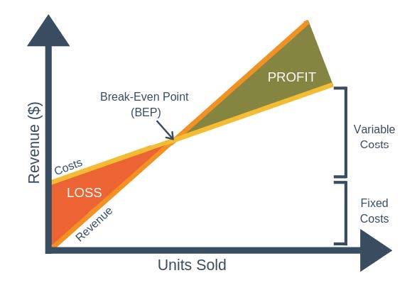
As output increases, variable costs are incurred, meaning that total costs (fixed + variable) also increase. At low levels of output, Costs are greater than Income. At the point of intersection, P, costs are exactly equal to income, and hence neither profit nor loss is made.
At this point it is important to differentiate between fixed and variable costs:
Fixed Costs
Fixed costs are those business costs that are not directly related to the level of production or output. In other words, even if the business has a zero output or high output, the level of fixed costs will remain broadly the same. In the long term fixed costs can alter – perhaps as a result of investment in production capacity (e.g. adding a new factory unit) or through the growth in overheads required to support a larger, more complex business. Examples of fixed costs: Rent and rates, Depreciation, Research and development and Administration costs.
Variable Costs
Variable costs are those costs which vary directly with the level of output. They represent payment output-related inputs such as raw materials, direct labour, fuel and revenue-related costs such as commission. A distinction is often made between “Direct” variable costs and “Indirect” variable costs.
Direct variable costs are those which can be directly attributable to the production of a particular product or service and allocated to a particular cost centre. Raw materials and the wages those working on the production line are good examples.
Indirect variable costs cannot be directly attributable to production but they do vary with output. These include depreciation (where it is calculated related to output – e.g. machine hours), maintenance and certain labour costs.
DRAWING A BREAK EVEN CHART
To draw a chart, the following steps, need to be followed:
- Label the vertical axis “sales and costs in Rands”.
- Label the horizontal axis “sales/production (units)”.
- On another piece of paper sketch, the scales that you want to use given the data, then use this plan on the chart.
- Plot any two points from the sales revenue data for the sales revenue line and then draw a straight line for sales revenue (assumes that the price per unit does not change) if the information is not given for sales revenue, then work out two points, e.g. for 1000 units sold and 1500 units sold. The start of the line should be through the origin (where the axes meet).
- Draw a horizontal line for total fixed costs starting at the point on the vertical axis at the level of costs.
- At the same starting point it is possible to draw the total costs line. Total costs are fixed costs plus variable costs. Work out what the total costs are for say 1000 units and 1500 units. Then draw the straight line starting at the same point as the fixed costs started and then through the two plotted points.
- Where the sales revenue crosses the total costs line is the breakeven point. Read off the units of sales to give the breakeven level of sales.
- The gap between the total costs line and sales revenue line after the breakeven point represents the level of profit.
WORKED EXAMPLE 2
A company producing a single article sells it at R 10 each. The variable cost of production is R. 6 each and fixed cost is R 400 per annum. Calculate the Breakeven point iN volume and sales;
400/(10-6)= 100 units
400/(10-6)= 100 units * 10
=R1, 000
WORKED EXAMPLE 3
A product sells for R15 and has variable costs per unit of R11. Each unit sale therefore makes a contribution of R4 towards the fixed costs of the business. If the business had fixed costs of R20, 000
Calculate the breakeven
Solution
200,000/ (15-11) = 5000 units